Mercury 2 Baseboard Applications

Let’s explore the potential of the Mercury 2 with the baseboard! These two tutorials will show off a few of the features of the baseboard, while giving a slightly more advanced Mercury 2 demo. It is recommended that you complete the Getting Started Guide, as this will walk you through design tool installation, project creation, and VHDL implementation using the Mercury 2 on its own. That guide will also be referenced heavily throughout this one. Information on the baseboard can be found here.

This page will be split up into two examples: first, an example using switch states as inputs to logic gates, with the results shown on the 7-segment display; second, an example using some more interesting features of the baseboard, such as the temperature and light sensors. The Mercury 2, in conjunction with the baseboard, is a very powerful tool with a myriad of applications.

XDC File for Baseboard Applications

Before starting with either example project, it is important to note that both projects use a specialized XDC file. This constraint set includes different pin definitions that are more readable when working on a project that uses baseboard features. As opposed to all of the IO pins being labeled “io(39 downto 0),” they have labels such as “sw(7 downto 0)” and “btn(3 downto 0)”. Since the projects below were created with this XDC in mind, they will not work with the typical Mercury XDC. Please download the baseboard XDC by clicking the button below.

Example 1: Digital Logic Gates

Step 1: Project Setup

To begin, download the VHDL files for the gates project. The source files are contained in a .zip folder for download here.

Once you have the files, loosely follow steps 1, 2, and 3 of the Getting Started Guide - there will be some differences detailed below. Once Vivado 2018.2 is installed, create the project. This example will use “gates4” as a project name, since it implements four unique logic gates. Be sure to leave the “Do not specify sources at this time” box unchecked.

Source files are added by clicking the “Add Files” button, navigating the explorer to where you unzipped the files for Gates4, and selecting all of the VHDL files.

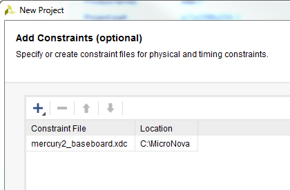
Once these steps are completed, Vivado gives the option of adding constraints. Add the Mercury Baseboard XDC file in the same way that the previous files were added.

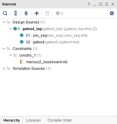
With this, project setup is complete. If new features are desired, changes can be made to the VHDL before generating a new .bit file. If the steps above were performed correctly, the Sources window in the Project Manager should look like this:

Step 2: Working With the Baseboard

Now that the project setup is successfully completed, the baseboard can be put to use. Go through Steps 5 and 6 in the Getting Started Guide, which go over creating and programming a *.bit file, so that the switches and 7-seg will talk to one another properly. Once these steps are complete, and the Mercury 2 is powered on, the baseboard should display a combination of 0s and 1s on the 7-seg depending on the switch positions. If SW0 through SW3 are pushed down, you should see something similar to the image below:

To understand what the board is actually displaying, look through gates4.vhd. The digits on the 7-segment display show AND, OR, XOR, and XNOR from left to right. The inputs to these logic gates are the four rightmost switches. Feel free to play around with the switches to see how each function reacts. The leftmost digit displays the logical result of SW0 & SW1 & SW2 & SW3. It will only display ‘1’ if all of the switches are high. The second digit displays the logical result of SW0 | SW1 | SW2 | SW3. It will display ‘1’ if at least one switch is high. The third digit displays exclusive or, also known as XOR. With only two inputs, this function is high if ONLY one of the inputs is high. With more than two inputs, it ends up being true when an ODD number of its inputs are true. This happens because the logical formula is something like: result = [(SW0 xnor SW1) xnor SW2] xnor SW3. The final digit displays exclusive nor, also known as XNOR. This is just the opposite of XOR, so it is high when an even number of its inputs are high or when none of them are high.

This example can be fun to play around with, and it can be expanded to other areas. All eight switches could be used for a slightly more complicated example, or real-world values can be fed into the logic gates. Changes to the VHDL files can make all of this possible.

Example 2: ADC Readings of Baseboard Sensors

Step 1: Project Setup

To begin, perform project setup similarly to Example 1. The same set of constraints will be used, so please download it using the link above if you haven’t already. Once again, the necessary VHDL files will be in a .zip folder for download below.

Once all of the files have been download, and project setup is complete, generate the .bit file and burn it to the board using the Mercury programming tool.

Step 2: Using the ADC to Interpret Real-World Data

ADC is short for analog-to-digital converter. As this is a 10-bit ADC, the device takes an analog voltage and converts it into a 10-bit binary number. Two of the three sensors that we interact with in this example function as voltage dividers - their resistance changes based on an input, which changes the output voltage. The temperature sensor is its own integrated circuit. In either case, the output goes from 0 volts to the value on VREF (ADC reference voltage), which translates to 0000000000 - 1111111111 (1023). This is typically around 5V because the Mercury 2 runs on 5V USB power and the sensors use the overall source voltage in their calculations; however, the reference voltage can be set to other values.

The temperature sensor ranges from about -20.5°C to 235.8°C according to the formula alone, but in reality, the range is about -10°C to 125°C. The specific formula used is Vout = (19.5mV/°C)*(Temp) + 400mV - calculations in the VHDL files are based on this formula. Depending on the season, the 7-segment display should show about 20-25°C at room temperature.

The light sensor and potentiometer are both a part of their own voltage divider. The light sensor sits between the ADC and our 5V source voltage. As brightness increases, the light sensor’s resistance decreases - this results in the ADC receiving a higher voltage from the sensor. Conversely, the resistance increases as it gets darker, so the voltage approaches 0V. The light sensor goes from roughly 5-10 kΩ at max brightness to 3 MΩ in pure darkness. It is being compared to a 4.7 kΩ resistor. Potentiometers form their own voltage dividers by literally splitting the resistor into two pieces. The output voltage will change depending on where the dial is positioned - turning clockwise decreases the voltage, while turning counter clockwise shows an increase.

With the Mercury 2 powered on, interpretations of sensor data should be shown on the 7-segment display. Starting with the temperature sensor (SW0 and SW1 low), three digits should be displayed. Typically, the first digit will be 0, and the remaining two will be the ambient temperature in °C. The leading digit will see use in really high and really low temperatures. Below 0°C, it will be used to show negative temperatures with “—”. Above 99°C, it will show “1” as expected. The temperature value can be manipulated by heating/cooling the sensor itself, which is located on the baseboard just below the USB connection point (ADC TEMP). The picture below is what you can expect to see in a typical case.

The light sensor only works with positive numbers - it is formulated so that the brightness scale goes from 0-100%. The sensor itself can be seen in the lower-left corner of the baseboard (ADC LIGHT). It can be difficult to get to 0% or 100%, but using flashlights or covering the sensor completely can provide those results. The three pictures below show different levels of brightness that should be easy to implement.

The potentiometer makes use of all three digits. The 7-segment display shows voltage with three significant digits. In the case of the picture below, the voltage is 3.11V. The scale runs from 0-5V, and the value can be changed by turning the dial next to the light sensor (ADC POT). This is very similar to adjusting the volume on a radio.

The sensors in this example follow the same basic format - read an outside stimulus, process that mathematically, and display it on the 7-seg. Plenty of other projects using the Mercury 2 could benefit from the baseboard sensors: temperature regulation could occur by running fans or other cooling devices based certain temperature thresholds; a robot on an assembly line could be alerted that inventory is low if the baseboard is installed below the parts and exposed to light when they’re removed; plenty of circuits can be controlled by adjusting voltage, basically giving you a small power supply.

The examples on this page merely scratch the surface of what the baseboard can do - hopefully they have inspired you to explore Mercury 2’s capabilities. The ADC, switches, buttons, and other peripherals can be used to create so much more!

For more information on the Mercury Baseboard, click here.

For more information on Mercury 2, click here.